 SensorPlot™ Hardware / Software SensorPlot™ Hardware / Software
 SensorPlot™ Hardware/Software Overview
The hardware of SensorPlot™ consists of a computer running Windows and one or more motion capture cards that facilitate the measurement position, velocity and acceleration. The computer and sensors are typically user supplied. Analog cards can also be plugged into the computer and cabled to the motion capture card(s) allowing you to make synchronous analog measurements.
The motion capture card is designed and manufactured by Euclid Research. It features:
The motion capture card is also sold independently from SensorPlot™ to data acquisition integrators building their own measurement systems.
Analog data acquisition cards: We currently re-sell National Instruments E series cards to support analog measurements. All cards support 16 single ended analog inputs or 8 differential analog inputs and are available in 12 and 16 bit versions. We also offer a number of signal condition modules.
SensorPlot™ Software Overview
SensorPlot™ is an integrated data acquisition and analysis system with particular emphasis on the analysis of mechanical motion. SensorPlot™ includes hardware data acquisition cards and a software application that runs under Microsoft Windows.
The system is operated like an instrument using menus and interactive controls. It requires no programming. The user is allowed to create arbitrary measurements by creating a number of displays, and associating user specified equations with these displays. When the instrument is run, measurements are made, equations are evaluated and the displays are updated.
This simplified tutorial discusses the software architecture and gives few examples of possible operations.
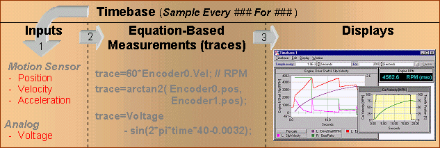
Below is a flow diagram illustrating the process of acquiring and displaying data:
Creating Measurements
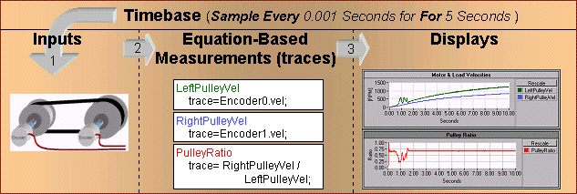
Let's start off by creating a simple velocity measurement on the input named Encoder0. All measurements in the system are represented by mathematical equations called traces. When you first begin, the traces you create typically reference the predefined measurements associated with the encoder inputs and analog inputs. These pre-defined measurements (called measurables) act like vector variables that are filled with samples as the system acquires data. A simple velocity measurement on the input named Encoder0 would like like:
| Trace Name | Trace Equation |
| LeftPulleyVel | Trace=Encoder0.vel; |
The .vel extension used in the equation above indicates that you want to use the velocity samples associated with Encoder0.
Because trace equations can reference the measurement results of other traces, creating a new measurement based on two underlying measurements involves nothing more than writing an equation. For example in the illustration below, the trace PulleyRatio simply references the other two measurements (LeftPulleyVel and RightPulleyVel) by their trace names.
You can also create more complex measurements in a single trace equation. For example, computing instantaneous power from measurements of voltage and current,
| Trace Name | Trace Equation |
| Power | Trace=Current * Voltage; |
or applying a moving average filter with an aperture of 16mS to remove a 60Hz component.
| Trace Name | Trace Equation |
| FilteredPower | Trace=MovingAvg( Current * Voltage, 1/60.0 ); |
To make life easier, SensorPlot™ includes many standard functions such as sin, cos, log, exp, and sqrt. The system also supports differentiation and integration functions, spectral analysis functions, variable and fixed aperture filters, and so on. Below is a sampling of what is available in the system:
Plotting Measurements
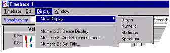
SensorPlot™ supports a variety of displays that can co-exist in any number. New displays can be dynamically created and destroyed through the Display menu of the Timebase as illustrated below.
Let's say you are plotting the trace PulleyRatio in it's own display, but you wish to plot it in the same display as the pulley velocity measurements. SensorPlot™ uses a common Add/Remove dialog box (shown below) to associate traces with a particular display. Adding the trace PulleyRatio to the graph plotting the pulley velocities involves nothing more than selecting the trace PulleyRatio from the User defined traces list, clicking on the Right Axis button (to add the trace to the right axis) and selecting OK.
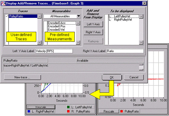
From this dialog box you can label the axis of a display, invoke the trace editor to create additional trace measurements, or simply add/remove measurements choosing from the measurements already defined. Because the system continuously evaluates all mathematical equations, new measurements are immediately evaluated and displayed as soon as they are added.
Editing Existing Measurements
To tools of SensorPlot™ have been designed to allow you to interactively analyze data during and after an acquisition. For example, clicking on the legend of a graph displays allows you to invoke a mini trace editor.
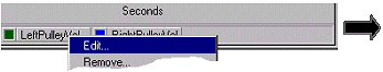 From this editor you can edit measurements without loosing data (e.g. add 60* to convert to RPM). Change the sign of the equation, scale it, or add functionality and the system immediately re-evaluates the equation and updates the appropriate displays. This instantaneous feedback allows you to interactively refine an experiment or diagnose a problem. | 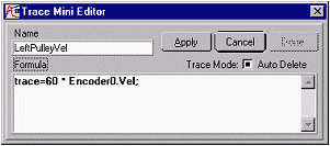 |
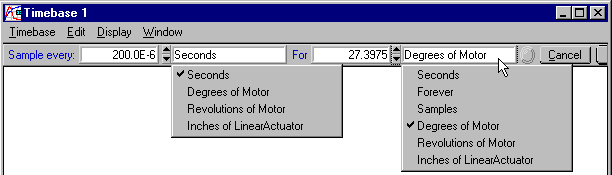
Sampling
The arrays (vectors) that hold the data for the measurables (pre-defined measurements) used in equations are filled with data at a rate dictated by the settings of the Timebase. The Timebase of SensorPlot™ is a hardware sampling sub-system that can be set to collect samples based on time, position or external event. The settings in the example below illustrate the acquisition of samples based on time for a length of time dictated by the angular position of a motor.
During an acquisition, measurables are filled with data and the equations that reference them are evaluated and displayed. The system evaluates equations incrementally as samples are acquired to ensure that the displays present data in real-time.
Saving To Files
Configurations can be saved on disk and retain complete system state including window positions, display configurations, equations, Timebase sampling parameters, input configurations (e.g. interface, termination) and so on. Saving all configuration information in the file allows experiments to be created for repeated use.
Saving With Data for Post-Analysis
Data that has been acquired can also be saved to disk for post analysis. The configuration associated with the collected data is also saved to preserve the context of the acquisition. Operations can be performed on the restored data as if it had just been acquired.
The same software that is used by the SensorPlot™ instrument also runs on a computer without the instrumentation hardware to allow post-acquisition data exploration to occur at a more convenient time and location (such as your quiet office).
Interactive Analysis Tools
SensorPlot™ supports a number of interactive analysis tools that allow you to explore the data once it has been acquired. These include:
Euclid Research · 2 North 1st Street, 6th Floor · San Jose, CA 95113-1201
Tel: (408) 283-9020 · Fax: (408) 283-9029